Interacting with naturaList: the map_module() function

Interactively exploring and editing occurrence data

In this article the user can explore the interactive module presented in naturaList package: the map_module() function. Through map_module() the user will be able to visual explore the occurrence data by seeing how it is distributed in space, as described in Figure 1.

Check out for records in a interactive map module

The map_module() function allow the user to visualize the occurrence records in a interactive map. To open the interactive module of naturaList package the user must provide an object containing occurrence records obtained from classify_occ function. To illustrate the usage of map module we will use the dataset containing the occurrences of Alsophila setosa and the list of specialist of tree ferns.

library(naturaList)
data("A.setosa") # occurrence points for A.setosa
data("speciaLists") # list of specialists for A.setosa

First we need to classify the occurrences of A. setosa through the classify_occ() function

occ.class <- classify_occ(A.setosa, speciaLists)

Now we can open the map module by providing the classification of A. setosa for map_module() function and save it in an object.

occ.select <- map_module(occ.class)

In this interactive map, the user can click over an occurrence point to see basic information about the record, such as the institution that holds the record, who identified the species and when it was identified. Also, if some error is identified, the user could allow that clicking works to delete points.

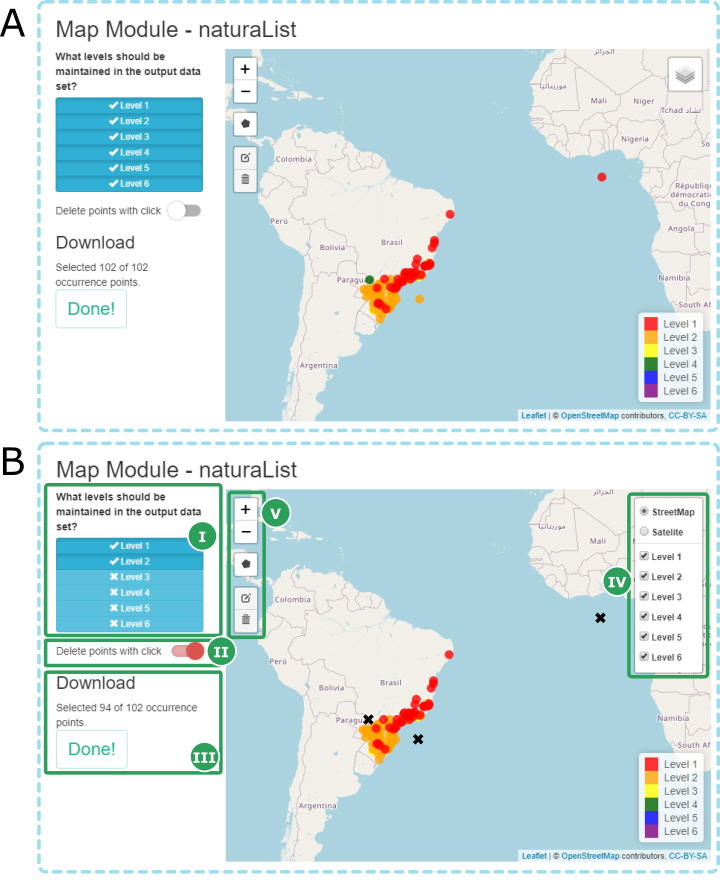
Fig. 1 - Features of map_module() function used in the example with Alsophila setosa occurrence data. A) the initial display of occurrence records data; B) highlights the features of map_module. I – Select levels to be maintained in the output dataset; II – enable to delete point with click over occurrences; III – show how many points have been selected from the initial dataset; IV – display in the map only occurrences that belong to the selected levels, and turn visualization of the map between OpenStreetMap and Satellite; V – options to draw and edit polygons to select occurrence records that fall within polygon; The “x” – represents a point deleted with click.

In the Figure 1, you see two screen shots from map_module(). In figure 1A, it is showed the initial display of occurrence records. In figure 1B it is highlighted the features inside map_module().

In this example, we selected the levels 1 and 2 (Fig 1B - I) to be shown in the module. We also deleted three records by setting on the button delete points with click (Fig 1B - II) and clicking on them. At the end of selection we click on ‘Done !’ button, that will close the map module and the modifications will be stored in occ_select object. The occ.select object corresponds to a data frame containing occurrences of A. setosa after the modification made with the map_module() function.

The map_module() also has the option to draw polygons to select various occurrences that fall inside the polygons. After the selection and click in the button Done! the points are saved in an object. In this example we selected four points using the draw polygon tool of map_module().

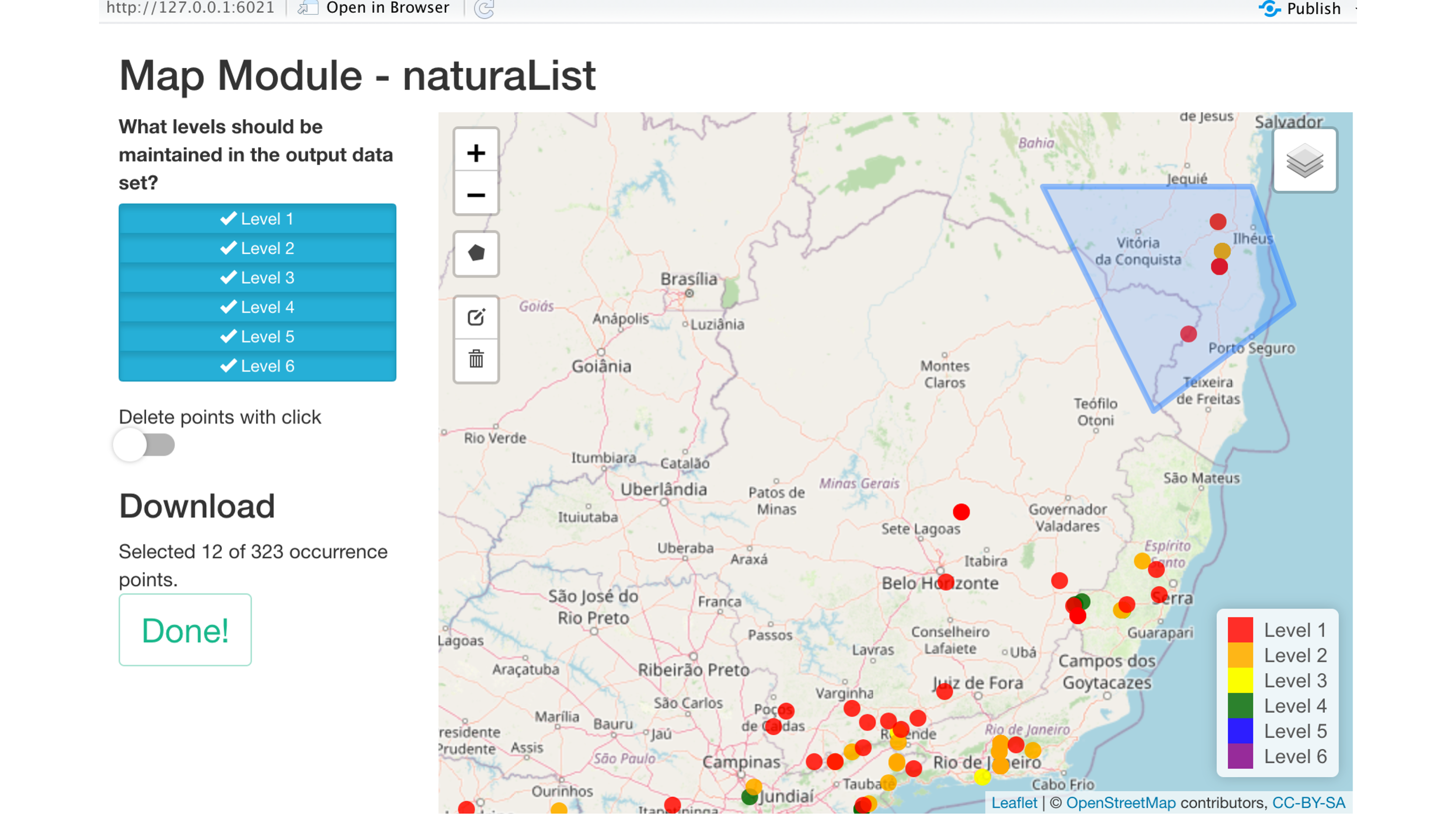
Fig. 2 - Draw polygon tool from map_module() function used in the example with Alsophila setosa occurrence data. In this example, the points inside the blue polygon were selected

The map_module() offers yet two options for the output dataset, which can be chosen in the argument action. If action = "clean" the output dataset contain only the occurrences selected by the user in the application. Otherwise, if action = "flag", the output dataset indicates which occurrence was selected and which was deleted by the user in the application. The flag option add a new column named map_module_flag to the output dataset, with the tags selected or deleted. By default the action = "clean". Check out the differences of this option:

occ.select1 <- map_module(occ.class, action = "flag")
occ.select2 <- map_module(occ.class, action = "clean")